If you see a circular reference warning in Excel, it usually points to a formula in a cell that, in some way, refers back to itself. As the formula can break its own result, this creates a circular reference. We’ll explain everything you need to know about circular references (and how to avoid or potentially use them) in this step-by-step guide.
You’ll see circular reference warnings for any formula you try to insert into Excel that loops back to itself. For instance, if you’re analyzing data with a SUMIF formula, and one of the cells in your data set is referencing the output from the same cell containing that formula, Excel can’t calculate the result, causing this error to appear.
However, there is one way you can use circular references in Excel to your advantage. If you want to insert an iterative calculation (one that repeats itself a limited number of times until certain conditions are met), you might want to use a circular reference formula, but you’ll need to tweak Excel’s settings to allow it.
Whether you’re looking to use circular references or avoid them entirely, this guide will explain:
- What are circular references in Excel and how do they work?
- How to quickly find and remove unwanted circular references in Excel
- How to enable iterative calculations in Excel
- How to create a circular reference formula in Excel
Are you struggling with circular references in Excel? Then keep reading!
1. What are circular references in Excel and how do they work?
For most users, a circular reference in Excel is problematic. Calculating the result of a formula, when the cell containing that formula is part of the calculation, results in an endless loop that Excel can’t complete.
Let’s use a very basic example. Let’s assume you have two cells: A2 and B2. Both contain references to the other cell, with A2 containing =B2, and B2 containing =A2. This is a circular reference, as the “formula” can’t be completed.
There isn’t an answer for Excel to output, so it displays an error. A blue arrow connecting the two cells offers a graphical representation of the problem.
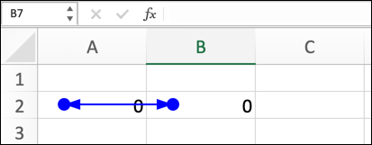
This also happens if, for example, you reference data in a cell that relies on the result of your first cell. For instance, A2 contains =B2, while B2 contains =C2. However, C2 contains a simple calculation, =A2-1. Because the overall result relies on the output of the initial cell (A2), this still results in an error.
Loops like these aren’t ideal for users working in an Excel workbook, largely because the excess calculations result in excessive memory usage (although the example above, by definition, wouldn’t result in any useful output anyway).
Excel won’t try to give you a result—the warning is sufficient to stop the error. Few users will want to disable it, but there is one advantage to doing so. If you decide you want to create a static result using functions that would otherwise change regularly, such as a timestamp, you could disable circular referencing to do so.
This is done by enabling iterative calculations, which are calculations that are repeated until certain conditions are met. Combined with certain logical functions, such as an IF function, you can turn otherwise volatile formulas into static ones that don’t update. This requires a bit of tweaking to Excel’s default settings, however.
Excel will throw up occasional errors with this kind of setting enabled, such as a zero output after quickly switching between selected cells. Where possible, it’s recommended to avoid this kind of scenario, or (at the very least) to limit the number of formulas where iterative calculations could cause data validity issues.
2. How to quickly find and remove unwanted circular references in Excel
Most users will want to avoid circular references appearing in their Excel workbooks. This is usually because it breaks the formula, preventing it from outputting a result (although a circular reference is, in many cases, a barrier to a result in the first place).
To get around this problem, you’ll need to locate and remove unwanted circular references in Excel. There are a couple of ways you can do this, from spotting the error symbol on certain cells to using Excel’s error checking system to locate them for you.
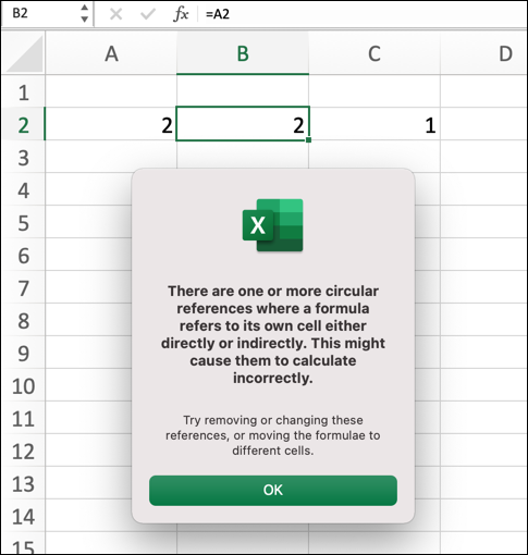
When you insert a formula that contains a circular reference in Excel, it will usually warn you. A pop-up will appear, along with a warning symbol alongside the cell itself. However, this pop-up and warning symbol won’t always appear if you’ve inserted multiple circular reference formulas into your workbook.
This can make finding each incorrect formula difficult, especially for larger data sets. To get around the problem, press the Formulas tab on the ribbon bar, then press the downwards arrow icon next to the Error Checking option. From the menu, hover over the Circular References option.
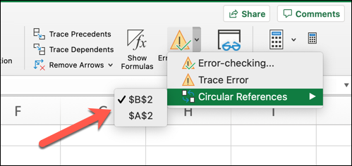
In the pop-up menu, you’ll see a list of absolute cell references to cells that contain formulas that cause circular references. Clicking on any of these cells causes Excel to find and select it in your workbook. You’ll also see the cell reference listed in the status bar at the bottom of the window.
Once you’ve located the cell, you’ll need to alter it to remove the circular reference and repeat this for each example of the problem in your workbook. Removing circular references from formulas will allow Excel to correctly return a result.
3. How to enable iterative calculations in Excel
Circular references are usually a sign that Excel is working as intended. If Excel tried to return a result where a circular reference existed, it would cause excessive memory usage and, depending on the formula, return incorrect results.
As we’ve mentioned, however, there is a limited exception to this rule where circular references are desirable. If you want to create static results from so-called volatile functions (such as time or date functions), you can use iterative calculations to do so.
Rather than creating a function that endlessly loops (potentially without success) to create a result, iterative calculations loop for a finite period of time. If the result is met, this creates a static result that doesn’t update. Excel isn’t really designed for this scenario, but it can work—just expect the odd error here and there.
If you want to enable iterative calculations in Excel 2010 and later, start by opening the Excel workbook containing your data. On Windows PCs, press File > Options, then select Formulas from the left-hand menu. Mac users should press Excel > Preferences > Calculation instead.
In the Formulas or Calculation menu (depending on your operating system), click to enable the Enable iterative calculation option. You’ll have two options you can change: maximum iterations and maximum change.
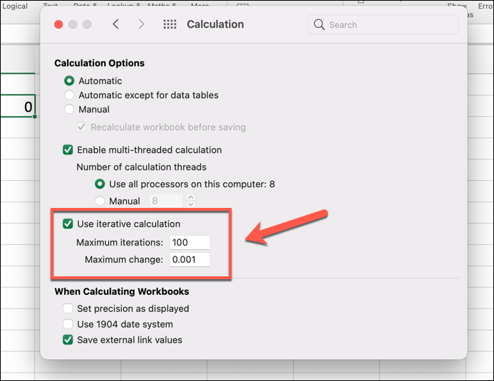
The maximum iterations value determines how often the formula should evaluate the result and potentially recalculate. Limiting or increasing this can increase or decrease the available time for a result to become viable. If a formula’s criteria isn’t met after the maximum value is passed, Excel will return zero as the result.
The maximum change value determines the accuracy of the output result, letting you decide how much a formula’s output can change before it stops recalculating. For instance, if the original value is 10 and the maximum change value is 0.1, and the value then changes to 10.1, Excel will stop recalculating, even if the maximum iterations value isn’t reached.
By default, Excel sets the maximum iterations value to 100 and the maximum change value to 0.001. You can increase or decrease these values to suit your own requirements.
To save the setting, press OK (on Windows) or close the settings menu (on Mac). The setting will apply to your open workbook specifically, and you’ll need to repeat these steps for any other workbook you wish to use.
4. How to create a circular reference formula in Excel: A step-by-step example guide using volatile and logical functions
If you’ve enabled iterative calculations in Excel, you can insert a formula that uses circular references into your Excel workbook. There’s no set formula to use, but we’ll demonstrate how it could prove effective by turning the output from volatile functions that update regularly (such as dates, times, or random numbers) into static results.
As we’ve mentioned, however, this kind of scenario has a very limited use case. Most users will probably want to avoid circular referencing like this to ensure the validity of your data. If you want to use it, however, you can follow these steps:
Step 1: Insert your initial data
Before you begin to insert a new formula, you’ll need to create a workbook and insert your data. For instance, you could create a table with a list of student names, where an iterative calculation could be used to show when a submission is received by creating a static timestamp.
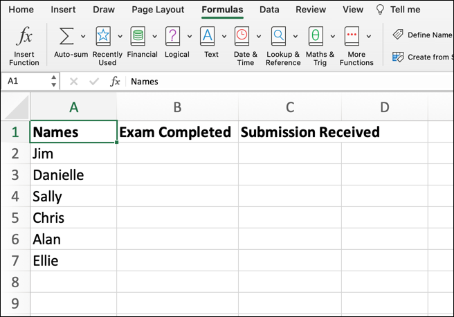
This is only one potential use case—you’ll need to determine the right data to use for your own workbook. Once you’ve inserted your data, you can move on to the next step.
Step 2: Select an empty cell
With your initial data inserted, you can begin to insert a new formula. To create a formula that creates static results from volatile results in a specific way, we’ll be creating a nested formula. This is a formula that combines more than one function.
To start, select an empty cell using your mouse. With the cell selected, press the formula bar at the bottom of the ribbon bar until you see the blinking cursor appear.
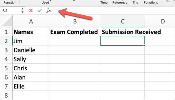
Once the blinking cursor is visible, you can begin to insert your formula.
Step 3: Insert your nested formula using volatile and logical functions
Logical functions (such as IF, SUMIF, OR, etc.) allow you to create formulas that only become visible when an argument is TRUE or FALSE. Combining this with a volatile function in a workbook with iterative calculations enabled allows you to create a static result from them.
Using our student lists example, we can create a static timestamp when an exam submission is received for each student. We’ll be using a nested IF formula to do this, but you could use any number of similar functions.
Logical tests like IF usually have three components: the test, the value if it’s true, and the value if it’s false. In this instance, the test is determining whether the rows in column B (for exam completion) have a YES or NO value. This is a TRUE/FALSE logical test. If YES is true, the static timestamp will appear, otherwise it won’t.
To create a function like this, type =IF(B2=”YES”,IF(C2=”“,NOW(),C2),””).
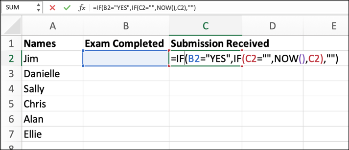
The IF formula in cell C2 checks whether the cell in B2 is equal to the text string YES. If it is, another nested IF formula checks to see if C2 is empty.
If it is, it’ll display a current timestamp using the NOW function, otherwise it’ll return an empty string (essentially a clever way to show the cell is empty). With iterative calculations active, this means that, when you insert YES into cell B2, the NOW() function will stop updating, creating a static timestamp.
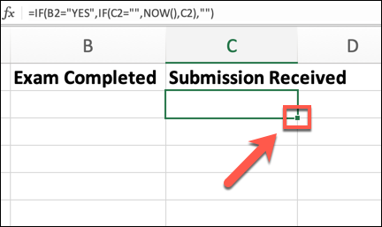
You can copy and paste your own formula into each cell to fill your column or press the green square icon in the bottom right corner of the selected cell to fill the column automatically.
Step 4: Satisfy the conditions for your formula
The purpose of this example formula is to demonstrate how iterative calculations can be used to create static results from volatile functions. NOW() is one example to show the current date and time, but you could also use RAND() for a random number, TODAY() for today’s date, etc.
You’ll need to first satisfy the conditions for your nested logical formula, however. To do this, select one of the cells in your test column, then insert the correct value for your formula test to become TRUE or FALSE, depending on your own formula.
In this instance, the cells in column B must contain YES. When you insert YES, the logical test becomes TRUE, creating a timestamp that, thanks to iterative calculations, won’t update.
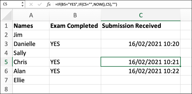
This is only one potential example. You can modify the steps above using your own data, different logical test formulas, and different test criteria to create static results from volatile functions that suit your own data.
Final thoughts
If you’re seeing circular reference warnings in Excel, it’s probably best to go through and fix them. However, if you’re keen to use circular references, you can combine volatile functions with logical tests to create static results using iterative calculations. Just remember that this isn’t how Excel is meant to operate, and can result in errors.
Watching out for circular references in your data is just one of several essential skills that new data analysts should watch out for in Excel. If you’ve already mastered the essential Excel formulas, you can take on a five-day short course to identify the other skills and experience you’ll need for a successful career in data analysis.
If you want to learn more about Excel or data analysis in general, you should check out these articles next:
