Spreadsheets are still in style! The use of electronic spreadsheets date back to 1979 and are still one of the most popular ways to review and manipulate data.
Today, Microsoft’s ubiquitous spreadsheet program Excel has over 750 million users and is used in some of the largest companies worldwide. I personally use Excel almost every day because it can sometimes lead to quicker results than spinning up Python or loading the data into a database.
One of the reasons Excel is so popular is because it is jam-packed with features and functions that can be used to clean, aggregate, pivot, and graph data. In this article, we’ll go over the 10 features and functions for using data analysis in Excel I think every analyst needs to know:
- Pivot tables and pivot charts
- Conditional formatting
- Remove duplicates
- XLOOKUP
- IFERROR
- MATCH
- COUNTBLANK
- DAYS and NETWORKDAYS
- RANK
- SUMPRODUCT
You can click any of the features to skip ahead to them.
Before we get started…
In order to show the power of data analysis in Excel, we need some data to play around with and graph. I am using the Customer Personality Analysis dataset from Kaggle in these examples. You can download it to follow along.

… and, if you want to watch along…
Here’s our very own senior data scientist, Tom, explaining these functions in a video:
1. Pivot tables and pivot charts
One of my favorite features in Excel is pivot charts and, as a close follow-up feature, pivot tables. Pivot charts visualize the data expressed in a pivot table, giving us insight at a glance. Pivot tables provide a simple approach to reformatting columns and rows, transforming them into groupings, statistics, or summaries. We can create a chart along with the table using the PivotChart feature under Insert.

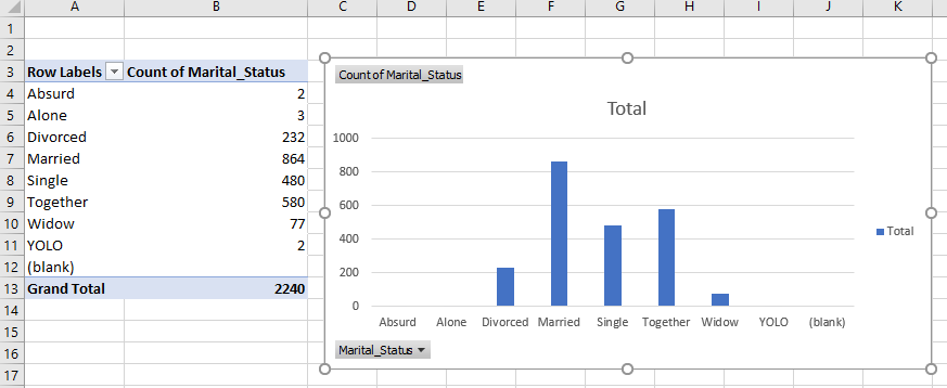
Let’s say we wanted to count the records grouped by Marital_Status. Using a pivot table makes that super simple, because it transforms the data and aggregates it for us.
To create a pivot chart and pivot table, first select the range of data you want to include then click Insert > PivotChart > PivotChart & PivotTable. The Create PivotTable editor will pop up.

The selected range will appear in the Table/Range field by default. Click OK and the pivot table will generate.

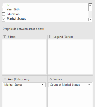
In the PivotChart Fields, drag Marital_Status from the field list into the Axis (Categories) box. Then drag Marital_Status from the field list into the Values box. Since the Marital_Status data is a string, the Values aggregation should default to Count. If the data type were numeric, the aggregation defaults to Sum.
The pivot table and chart should populate. You can add additional dimensions or filters by dragging new fields into the corresponding box. It only takes a few clicks to aggregate data and visualize it in Excel, which is why it is such a widely-used tool.
2. Conditional formatting
Thinking about it, I probably use conditional formatting more than any other feature in Excel. Conditional formatting allows you to highlight or hide cells based on a rule you specify. Apply the rules to one cell or multiple cells in the same worksheet. It is useful for highlighting outliers, duplicates, or patterns in data.

Let’s say we want to highlight all Year_Birth values greater than 1987 in the dataset.
Select the Year_Birth column and click Conditional Formatting > Highlight Cells Rules > Greater Than. The editor will pop up:

Enter 1987 and click OK. The cells in the column with a value greater than 1987 will turn light red.
If we decide we want to adjust the conditional formatting rule we just created, follow path Conditional Formatting > Conditional Formatting Rules Manager.

From the manager we are able to create new rules or edit existing ones. It is possible to have multiple rules affecting the spreadsheet.
3. Remove duplicates
Data is often messy, so it is important that you know how to remove duplicates. Using conditional formatting rules, you can highlight the duplicate data to review it before deleting it. The Remove Duplicates feature is available under Data > Data Tools > Remove Duplicates.
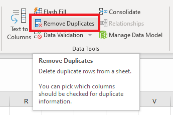
Highlight the dataset in Excel and click Remove Duplicates. The Remove Duplicates editor appears:
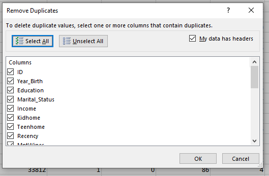
The editor allows us to select columns that should be included when deleting the duplicates. Make sure the My data has headers checkbox is marked if the column names are not displaying.
Click OK. The duplicates will be dropped from the dataset. It will tell us how many unique values remain.
4. XLOOKUP
XLOOKUP is like a combination of VLOOKUP and HLOOKUP, since it can go either vertically or horizontally to lookup a value from a range. It essentially allows you to use a selected range as a lookup table and return a “looked up” result to a cell. The syntax is as follows:
=XLOOKUP(lookup_value, lookup_array, return_array, [if_not_found], [match_mode], [search_mode])
Let’s say we want to look up the Year_Birth based on an entered ID value. In cell AD2, enter an ID value—for example, 8755. In cell AE2, enter the XLOOKUP formula:
=XLOOKUP(
The lookup_value is the value we want looked up by the function, so we enter AD2.
The lookup_array is a column or row that contains the lookup value, so we enter A2:A2241 since that will give us an array of IDs.
The return_array is the column or row that contains the value we want to return, so we select B2:B2241 since that will give us Year_Birth values.
The completed formula will look like this: =XLOOKUP(AD2, A2:A2241, B2:B2241)

Enter in different IDs and the corresponding Year_Birth will return.
Lookup functions are very powerful, and you can even join data from different sheets or nest lookup functions within each other. For example, you could sum the value of multiple lookups.
5. IFERROR
The IFERROR function is used to create a custom error message when a formula results in an error. For example, we can use it to wrap our XLOOKUP function so it returns a clear message if the ID isn’t found. The syntax is relatively simple.
=IFERROR(value, value_if_error)
Going back to the XLOOKUP function, if we enter an ID in to AD2 that doesn’t exist in the lookup array, AE2 outputs #N/A. Instead, let’s return “ID Not Found.” For the value in the IFERROR function, use the XLOOKUP function. It should look like this:
=IFERROR(XLOOKUP(AD2, A2:A2241, B2:B2241), “ID Not Found”)

In addition to text, you can point the value_if_error at another cell too. If you target a blank cell as the value for value_if_error, 0 will appear in the cell.
6. MATCH
Similar to the lookup functions, MATCH can be used when you need the position of a value in a range instead of the value itself.
This is the syntax for MATCH:
=MATCH(lookup_value, lookup_array, [match_type])
When writing the function, it is important to know which match type to use. Although it is optional and defaults to 1, the available options are -1, 0, or 1.
- -1: Finds the smallest value that is greater than or equal to lookup_value.
- 0: Finds the first value that is exactly equal to lookup_value.
- 1: Finds the largest value that is less than or equal to lookup_value.
If we want to find the first time the looked up birth year occurs, add a the following MATCH formula to cell AF2:
=MATCH(AE2,B:B, 0)

7. COUNTBLANK
The COUNTBLANK function is fairly intuitive, but it is an important function for data wrangling in analytics because many machine learning algorithms are sensitive to nulls. By knowing how many values are null, you have a better understanding of how to approach them. For example, if a lot of values are null you should drop the column. If few values are null you should impute a value to fill the null. COUNTBLANK counts the number of empty cells in a range. The syntax is simple:
=COUNTBLANK(range)
We want to count the number of nulls in the Income column, so add this formula to cell AG2:
=COUNTBLANK(E2:E2241)

8. DAYS and NETWORK DAYS
DAYS and NETWORKDAYS are separate functions, but they are similar enough to not warrant individual entries in my list. The DAYS function simply returns the number of days between two dates, whereas the NETWORKDAYS function is slightly different in that it excludes weekends and specified holidays. It only returns the number of working days between two dates. The syntax for both is easy to remember:
=DAYS(start_date, end_date)
=NETWORKDAYS(start_date, end_date, [holidays])
At my job, one of the things I analyze is usage data. I use these functions for things like counting the number of days since a user has logged in or used a tool. Since our software is used in schools, sometimes it makes sense to exclude weekends and holidays from our usage data so I’m thankful for the NETWORKDAYS function.
9. RANK
The RANK function orders a number by its size relative to other values in a list and returns the desired rank. That means the rank of the number would be its position if the list becomes sorted by ascending or descending order. For example, sort Income in descending order so the biggest value is at the top and that could be rank 1. RANK gives duplicate numbers the same rank, but cumulatively counts. That means if two values are rank four, the next rank will be six, not five (1,2,3,4,4,6). The syntax for RANK takes 3 arguments.
=RANK(number, ref, [order])
It is important to note that [order] can be set to 0 for descending and 1 (or greater) for ascending.
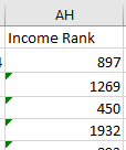
We want to rank the income (column E) of our customers, so we will use the following formula in cell AH2:
=RANK(E2, E2:E2241, 0)
In the bottom right corner of cell AH2, click the square and drag it down to the last row of data and the formula will automatically copy allowing us to quickly generate a rank for each income value.
10. SUMPRODUCT
The last function on my top 10 list is SUMPRODUCT. It is great when you need to do arithmetic on specific groups of values. It can be used to add, subtract, multiply or divide the selected numerical values for corresponding ranges. Although it sounds complicated, the logic is fairly intuitive once you try it. The syntax, however, is not very intuitive.
=SUMPRODUCT(array1, [array2], [array3], …)
We want to sum the KidHome for all rows where Education equals Graduation (C2) and Marital_Status equals Single (D2). We will add this formula to cell AI:
=SUMPRODUCT((C2:C2241=C2)*(D2:D2241=D2)*(F2:F2241))

If we wanted to see a different Education value, PhD for example, we could change C2 to C6 in the formula.
Summary and next steps
This is by no means an exhaustive list of every feature and function Excel offers, but these 10 functions help me analyze and clean data without the hassle of booting up Python or loading the data in a SQL server.
Pivot charts are great for small data sets, especially if you need to share the data with non-technical people. Even though Excel seems like a cumbersome tool in a world of big data, it remains one of the most popular data analytics tools on the planet for a reason.
But don’t take our word for it—CareerFoundry Data Analytics Program graduate Nick had this advice for other potential career-changers, after successfully completing his move from math teacher to data analyst:
To know Excel—no matter what your role—is important. If you work at a business and you know some of the more intermediate-to-advanced Excel skills, it’s going to help save you time, and maybe even come up with something that’s going to impress your boss. Excel is a huge tool that is a lot more robust than I knew it to be.
If you’d like to learn more about data analytics, try out this free 5-day short course, or check out some of our other data analytics articles:
