There are a few different ways to insert symbols in Excel. These include using your computer’s keyboard, buttons on the Ribbon, a formula, and cell formatting.
A symbol that is commonly used in Excel is the Delta symbol. This is often found on Excel dashboards and scorecards to present a change in values.
In this article, we’ll show you three different methods to insert the Delta symbol. We’ll also explain the differences between each method and why you may choose one method over another in a given situation.
You can more Excel analysis skills by trying CareerFoundry’s free 5-day data short course.
We’ll cover:
- What is the Delta symbol?
- How to insert the Delta symbol
- How to type the Delta symbol
- Custom Number Formatting to show the Delta symbol
- Key takeaways
You can use this Excel workbook to follow along with the examples in this article.
So, let’s dive into the different methods for inserting the Delta symbol.
1. What is the Delta symbol?
The Delta symbol is the fourth character in the Greek alphabet. In mathematics, it means ‘change’. So, ∆x means ‘change in x’.
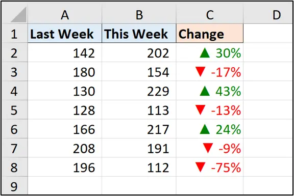
In Excel, the symbol is used to visualize a change in values. It is often filled in and colored in either green or red to visualize a positive or negative change clearly to the reader.
2. How to insert the Delta symbol
The easiest way to insert the Delta symbol is using the symbols library. This is also common to many Office products, and is not a technique restricted to Excel use only.
- Click in the cell where you want to insert the symbol.
- Click Insert > Symbols > Symbol.
- Change the Font list to a typical writing font, if necessary, such as Arial or Calibri.
- From the Subset list, select Greek and Coptic.
- Locate and click on the Delta symbol. You will see the unicode name appear in the bottom left of the window as “Greek Capital Letter Delta”.
- Click Insert.
The Delta symbol is inserted in the selected cell.
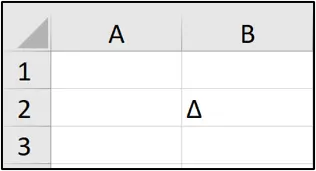
Now, this is the Delta symbol, but when using Excel it is preferred to use a filled upwards-pointing triangle instead.
- Click in the cell where you want to insert the symbol, and click Insert > Symbols > Symbol.
- Select Wingdings 3 from the Font list.
- Locate and click on the “Black Up-Pointing Triangle” symbol.
You can see in the following image that the symbols appear in my Recently used symbols at the bottom of the window.
This makes it fast and easy to insert again in the future. You will not need to find them every time, if you use them often.
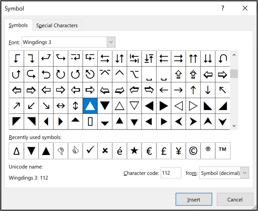
4. Click Insert.
The “Black Up-Pointing Triangle” is inserted to the selected cell.
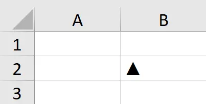
This method is quick and simple, but the process requires repeating every time the symbol needs inserting. We will see an automated solution soon when we display the Delta symbol using number formatting.
3. How to type the Delta symbol
Another option when you just need to enter the Delta symbol quickly, is to type it. Now, this is only if you have a keyboard with a number pad.
To type the Delta symbol, you first need to make sure that you have the Num Lock on to activate the numbers in the number pad. Then press and hold the Alt key and type 30.
Alt + 30 is the keyboard sequence to enter the Delta symbol. Or to be more precise, it inserts the preferred “Black Up-Pointing Triangle” symbol.
4. Custom Number Formatting to show the Delta symbol
Using custom number formatting in Excel to insert the Delta symbol provides an effective method for your Excel dashboards.
The number formatting can be used to display the appropriate symbol depending on the change in values. An up triangle to indicate the value has increased, and a down triangle if the value has decreased.
The image below shows two columns of values: last week and this week. We also have another column with the percent variance calculated.
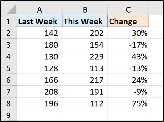
We will use number formatting to display the up or down triangle symbol before the percent values in column C.
- Select the values you want to format, range C2:C8 in this example.
- Press Ctrl +1, or right click and click Format Cells.
- From the Number tab, click Custom in the Category list.
- Type the following code into the Type field.
[Green] ▲ 0%;[Red] ▼ -0%
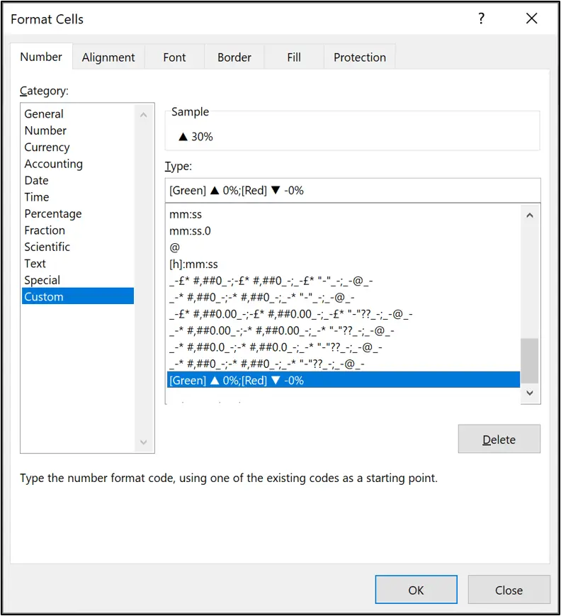
There is quite a lot happening here if you are new to custom number formatting. So, let’s explain a few things.
The semicolon “;” in the code separates the positive and negative formats. The code before the semicolon specifies how positive numbers should be displayed, and after the semicolon is for negative numbers.
For the triangle symbols, you will not be able to insert these when in the Format Cells window. Best practise is to insert them into the worksheet as demonstrated earlier in the article, copy them to the clipboard and then paste them into the Type field of Format Cells.
The names of colors in the square brackets format the font. Only a few colors can be specified by their name.
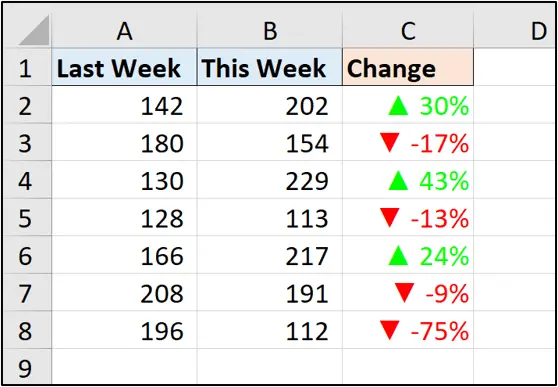
I don’t like the green color that the name provides, so instead I use a color number. The color number 10 is a better green in my opinion.
The following code can be used instead.
[Color10] ▲ 0%;[Red] ▼ -0%
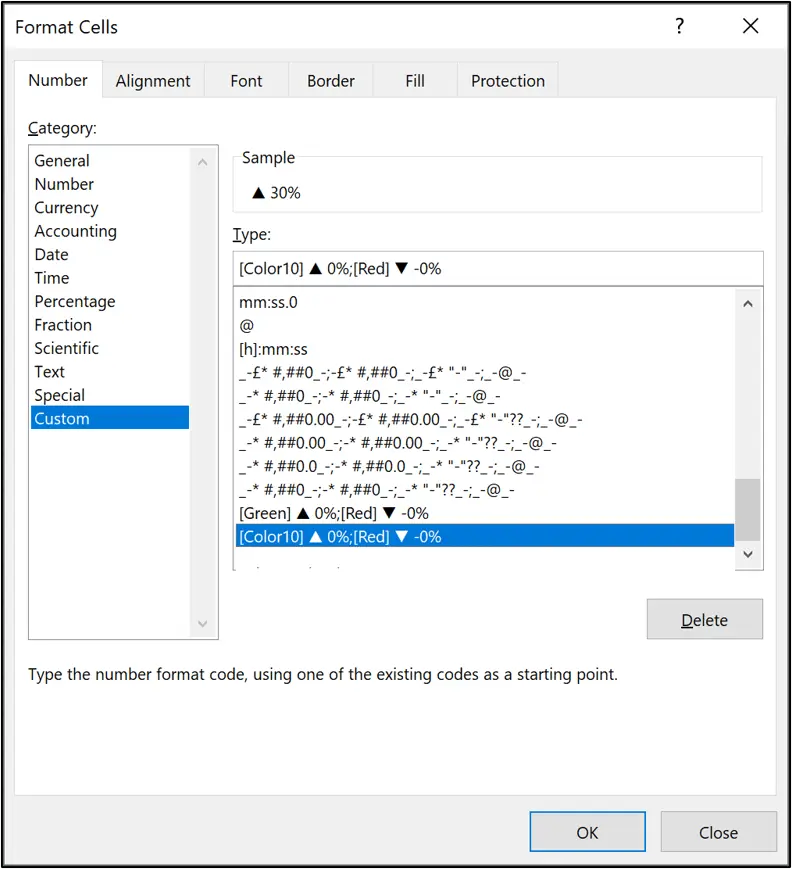
The percent variance values are now presented effectively.
The filled triangles provide a better symbol than the official Delta symbol in Excel and portray the same meaning of ‘change’.

6. Key takeaways
In this article, we shared three methods for inserting the Delta symbol, or filled triangles, in Excel.
- Insert symbols using the Ribbon. This is quick and simple, but not a good solution if the values change often.
- Type the Delta symbol using Alt + 30. This method requires a keyboard with a number pad.
- Insert symbols using number formatting. This is the most flexible approach and ideal for dashboards. The triangles change automatically as the values change and you can build in extra conditions if required.
Understanding the different methods for inserting symbols such as Delta in Excel provides you with the skills to present data effectively in different situations.
For a hands-on introduction to the field of data analytics, try out this free five-day short course. And, for more Excel tutorials, check out the following:
