All statistical techniques can be divided into two broad categories: descriptive and inferential statistics. In this post, we explore the differences between the two, and how they impact the field of data analytics.
Statistics. They are the heart of data analytics. They help us spot trends and patterns. They help us plan. In essence, they breathe life into data and help us derive meaning from it.
While the individual statistical methods we use in data analytics are too numerous to count, they can be broadly divided into two main camps: descriptive statistics and inferential statistics. In this post, we explore the difference between descriptive and inferential statistics, and touch on how they’re used in data analytics. We’ll break things down into the following bite-sized chunks:
- What is statistics?
- What’s the difference between inferential and descriptive statistics?
- Must know: What are population and sample?
- What is descriptive statistics?
- What is inferential statistics?
- Inferential vs descriptive statistics FAQs
Ready? Engage!
1. What is statistics?
Put simply, statistics is the area of applied math that deals with the collection, organization, analysis, interpretation, and presentation of data.
Sound familiar? It should. These are all vital steps in the data analytics process. In fact, in many ways, data analytics is statistics. When we use the term ‘data analytics’ what we really mean is ‘the statistical analysis of a given dataset or datasets’. But that’s a bit of a mouthful, so we tend to shorten it!
Since they are so fundamental to data analytics, statistics are also vitally important to any field that data analysts work in. From science and psychology to marketing and medicine, the wide range of statistical techniques out there can be broadly divided into two categories: descriptive statistics and inferential statistics. But what’s the difference between them?
In a nutshell, descriptive statistics focus on describing the visible characteristics of a dataset (a population or sample).
Meanwhile, inferential statistics focus on making predictions or generalizations about a larger dataset, based on a sample of those data.
2. What’s the difference between inferential and descriptive statistics?
Let’s look at an overview of the differences between these two categories:
Descriptive statistics:
- Describe the features of populations and/or samples
- Organize and present data in a purely factual way
- Present final results visually, using tables, charts, or graphs
- Draw conclusions based on known data
- Use measures like central tendency, distribution, and variance
Inferential statistics:
- Use samples to make generalizations about larger populations
- Help us to make estimates and predict future outcomes
- Present final results in the form of probabilities
- Draw conclusions that go beyond the available data
- Use techniques like hypothesis testing, confidence intervals, and regression and correlation analysis
Important note: while we’re presenting descriptive and inferential statistics in a binary way, they are really most often used in conjunction.
3. What are population and sample in statistics?
Before we go explore these two categories of statistics further, it helps to understand the vital concepts of what population and sample mean. We can define them as follows:
Population
This the entire group that you wish to draw data from (and subsequently draw conclusions about).
While in day-to-day life, the word is often used to describe groups of people (such as the population of a country) in statistics, it can apply to any group from which you will collect information. This is often people, but it could also be cities of the world, animals, objects, plants, colors, and so on.
A sample
This a representative group of a larger population. Random sampling from representative groups allows us to draw broad conclusions about an overall population.
This approach is commonly used in polling. Pollsters ask a small group of people about their views on certain topics. They can then use this information to make informed judgments about what the larger population thinks. This saves time, hassle, and the expense of extracting data from an entire population (which for all practical purposes is usually impossible).

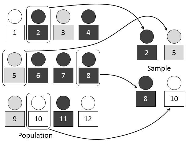
Attribution: Dan Kernler, CC BY-SA 4.0, via Wikimedia Commons
The image illustrates the concept of population and sample. Using random sample measurements from a representative group, we can estimate, predict, or infer characteristics about the larger population. While there are many technical variations on this technique, they all follow the same underlying principles.
OK! Now we understand the concepts of population and sample, we’re ready to explore descriptive and inferential statistics in a bit more detail.
4. What is descriptive statistics?
Descriptive statistics are used to describe the characteristics or features of a dataset. The term “descriptive statistics” can be used to describe both individual quantitative observations (also known as “summary statistics”) as well as the overall process of obtaining insights from these data.
We can use descriptive statistics to describe both an entire population or an individual sample. Because they are merely explanatory, descriptive statistics are not heavily concerned with the differences between the two types of data.
So what measures do descriptive statistics look at? While there are many, important ones include:
- Distribution
- Central tendency
- Variability
Let’s briefly look at each of these now.
What is distribution?
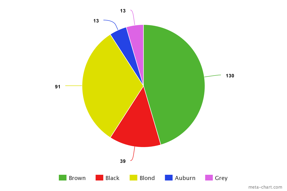
Distribution shows us the frequency of different outcomes (or data points) in a population or sample. We can show it as numbers in a list or table, or we can represent it graphically. As a basic example, the following list shows the number of those with different hair colors in a dataset of 286 people.
- Brown hair: 130
- Black hair: 39
- Blond hair: 91
- Auburn hair: 13
- Gray hair: 13
We can also represent this information visually, for instance in a pie chart.

Generally, using visualizations is common practice in descriptive statistics. It helps us more readily spot patterns or trends in a dataset.
What is central tendency?
Central tendency is the name for measurements that look at the typical central values within a dataset. This does not just refer to the central value within an entire dataset, which is called the median. Rather, it is a general term used to describe a variety of central measurements. For instance, it might include central measurements from different quartiles of a larger dataset. Common measures of central tendency include:
- The mean: The average value of all the data points.
- The median: The central or middle value in the dataset.
- The mode: The value that appears most often in the dataset.
Once again, using our hair color example, we can determine that the mean measurement is 57.2 (the total value of all the measurements, divided by the number of values), the median is 39 (the central value) and the mode is 13 (because it appears twice, which is more than any of the other data points).
Although this is a heavily simplified example, for many areas of data analysis these core measures underpin how we summarize the features of a data sample or population. Summarizing these kinds of statistics is the first step in determining other key characteristics of a dataset, for example, its variability. This leads us to our next point…
What is variability?
The variability, or dispersion, of a dataset, describes how values are distributed or spread out. Identifying variability relies on understanding the central tendency measurements of a dataset. However, like central tendency, variability is not just one measure. It is a term used to describe a range of measurements. Common measures of variability include:
- Standard deviation: This shows us the amount of variation or dispersion. Low standard deviation implies that most values are close to the mean. High standard deviation suggests that the values are more broadly spread out.
- Minimum and maximum values: These are the highest and lowest values in a dataset or quartile. Using the example of our hair color dataset again, the minimum and maximum values are 13 and 130 respectively.
- Range: This measures the size of the distribution of values. This can be easily determined by subtracting the smallest value from the largest. So, in our hair color dataset, the range is 117 (130 minus 13).
- Kurtosis: This measures whether or not the tails of a given distribution contain extreme values (also known as outliers). If a tail lacks outliers, we can say that it has low kurtosis. If a dataset has a lot of outliers, we can say it has high kurtosis.
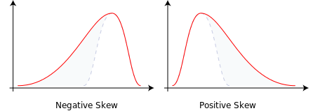
- Skewness: This is a measure of a dataset’s symmetry. If you were to plot a bell-curve and the right-hand tail was longer and fatter, we would call this positive skewness. If the left-hand tail is longer and fatter, we call this negative skewness. This is visible in the following image.

Attribution: Rodolfo Hermans (Godot) at en.wikipedia., CC BY-SA 3.0, via Wikimedia Commons
Used together, distribution, central tendency, and variability can tell us a surprising amount of detailed information about a dataset. Within data analytics, they are very common measures, especially in the area of exploratory data analysis. Once you’ve summarized the main features of a population or sample, you’re in a much better position to know how to proceed with it. And this is where inferential statistics come in.
Want to try your hand at calculating descriptive statistics? In this free data analytics tutorial, we show you, step by step, how to calculate the mean, median, mode, and frequency for certain variables in a real dataset as part of exploratory data analysis. Give it a go!
So, we’ve established that descriptive statistics focus on summarizing the key features of a dataset. But what about inferential ones?
5. What is inferential statistics?
Inferential statistics focus on making generalizations about a larger population based on a representative sample of that population. Because inferential statistics focuses on making predictions (rather than stating facts) its results are usually in the form of a probability.
Unsurprisingly, the accuracy of inferential statistics relies heavily on the sample data being both accurate and representative of the larger population. To do this involves obtaining a random sample. If you’ve ever read news coverage of scientific studies, you’ll have come across the term before. The implication is always that random sampling means better results.
On the flipside, results that are based on biased or non-random samples are usually thrown out. Random sampling is very important for carrying out inferential techniques, but it is not always straightforward!
Let’s quickly summarize how you might obtain a random sample.
How do we obtain a random sample?
Random sampling can be a complex process and often depends on the particular characteristics of a population. However, the fundamental principles involve:
1. Defining a population
This simply means determining the pool from which you will draw your sample. As we explained earlier, a population can be anything—it isn’t limited to people. So it could be a population of objects, cities, cats, pugs, or anything else from which we can derive measurements!
2. Deciding your sample size
The bigger your sample size, the more representative it will be of the overall population. Drawing large samples can be time-consuming, difficult, and expensive. Indeed, this is why we draw samples in the first place—it is rarely feasible to draw data from an entire population. Your sample size should therefore be large enough to give you confidence in your results but not so small that the data risk being unrepresentative (which is just shorthand for inaccurate). This is where using descriptive statistics can help, as they allow us to strike a balance between size and accuracy.
3. Randomly select a sample
Once you’ve determined the sample size, you can draw a random selection. You might do this using a random number generator, assigning each value a number and selecting the numbers at random. Or you could do it using a range of similar techniques or algorithms (we won’t go into detail here, as this is a topic in its own right, but you get the idea).
4. Analyze the data sample
Once you have a random sample, you can use it to infer information about the larger population. It’s important to note that while a random sample is representative of a population, it will never be 100% accurate. For instance, the mean (or average) of a sample will rarely match the mean of the full population, but it will give you a good idea of it. For this reason, it’s important to incorporate your error margin in any analysis (which we cover in a moment). This is why, as explained earlier, any result from inferential techniques is in the form of a probability.
However, presuming we’ve obtained a random sample, there are many inferential techniques for analyzing and obtaining insights from those data. The list is long, but some techniques worthy of note include:
- Hypothesis testing
- Confidence intervals
- Regression and correlation analysis
Let’s explore a bit more closely.
What is hypothesis testing?
Hypothesis testing involves checking that your samples repeat the results of your hypothesis (or proposed explanation). The aim is to rule out the possibility that a given result has occurred by chance. A topical example of this is the clinical trials for the Covid-19 vaccine. Since it’s impossible to carry out trials on an entire population, we carry out numerous trials on several random, representative samples instead.
The hypothesis test, in this case, might ask something like: ‘Does the vaccine reduce severe illness caused by covid-19?’ By collecting data from different sample groups, we can infer if the vaccine will be effective.
If all samples show similar results and we know that they are representative and random, we can generalize that the vaccine will have the same effect on the population at large. On the flip side, if one sample shows higher or lower efficacy than the others, we must investigate why this might be. For instance, maybe there was a mistake in the sampling process, or perhaps the vaccine was delivered differently to that group.
In fact, it was due to a dosing error that one of the Covid vaccines actually proved to be more effective than other groups in the trial… Which shows how important hypothesis testing can be. If the outlier group had simply been written off, the vaccine would have been less effective!
What is a confidence interval?
Confidence intervals are used to estimate certain parameters for a measurement of a population (such as the mean) based on sample data. Rather than providing a single mean value, the confidence interval provides a range of values. This is often given as a percentage. If you’ve ever read a scientific research paper, conclusions drawn from a sample will always be accompanied by a confidence interval.
For example, let’s say you’ve measured the tails of 40 randomly selected cats. You get a mean length of 17.5cm. You also know the standard deviation of tail lengths is 2cm. Using a special formula, we can say the mean length of tails in the full population of cats is 17.5cm, with a 95% confidence interval. Essentially, this tells us that we are 95% certain that the population mean (which we cannot know without measuring the full population) falls within the given range. This technique is very helpful for measuring the degree of accuracy within a sampling method.
What are regression and correlation analysis?
Regression and correlation analysis are both techniques used for observing how two (or more) sets of variables relate to one another.
Regression analysis aims to determine how one dependent (or output) variable is impacted by one or more independent (or input) variables. It’s often used for hypothesis testing and predictive analytics. For example, to predict future sales of sunscreen (an output variable) you might compare last year’s sales against weather data (which are both input variables) to see how much sales increased on sunny days.
Correlation analysis, meanwhile, measures the degree of association between two or more datasets. Unlike regression analysis, correlation does not infer cause and effect. For instance, ice cream sales and sunburn are both likely to be higher on sunny days—we can say that they are correlated. But it would be incorrect to say that ice cream causes sunburn! You can learn more about correlation (and how it differs from covariance) in this guide.
What we’ve described here is just a small selection of a great many inferential techniques that you can use within data analytics. However, they provide a tantalizing taste of the sort of predictive power that inferential statistics can offer.
6. Descriptive vs inferential statistics FAQs
What is an example of a descriptive statistic?
A good example would be a pie chart displaying the different hair colors in the population, clearly showing that brown hair is the most common.
Should I use descriptive or inferential statistics?
Which to use depends on the situation, as they have different goals. In general, descriptive statistics are easier to carry out and are generalizations, and inferential statistics are more useful if you need a prediction. So, it depends on the scenario and what you yourself are looking for.
What is an example of an inferential statistic?
This would be analyzing the hair color of one college class of students and using that result to predict the most popular hair color in the entire college.
7. Wrap-up
So there you have it, everything you need to know about descriptive vs inferential statistics! Although we examined them separately, they’re typically used at the same time. Together, these powerful statistical techniques are the foundational bedrock on which data analytics is built.
To learn more about the role that descriptive and inferential statistics play in data analytics, check out our free, 5-day short course. If that’s piqued your interest in pursuing data analytics as a career, why not then check out the best online data analytics courses on the market? For more introductory data analytics topics, see the following:
