If you’re learning Python for data analytics, odds are you’ve heard of the pandas library. Back when I first started to learn data analytics, the first tool I used was spreadsheets, since I didn’t know how to code.
Although tools like Excel and Google Sheets are powerful, spreadsheets become difficult to use when handling large datasets and can quickly feel cumbersome or run out of memory. If you have to work with big data containing millions or billions of records, Python is a much better tool for the job.
Pandas is one of the most popular Python libraries for handling data, and is widely used in analytics, data science, and finance because of its robust functionality and ability to process data quickly. Created by Wes McKinney, the Pandas library has remained open source and has a solid community that is regularly updating the package.
In this article we’re going to walk through a Python pandas tutorial so you have a better understanding of how and when to use it. We’ll cover the following topics in this article:
- How do data analysts use pandas?
- An introduction to Series and DataFrame
- Python pandas tutorial: Installing pandas
- Python pandas tutorial: Series
- Python pandas tutorial: DataFrame
- Next steps
This article assumes you already have a basic understanding of the Python programming language. Check out this article if you’re new to Python and want to learn more about it.
1. How do data analysts use pandas?
Before getting into the Python pandas tutorial code examples, let’s review how data analysts use the Pandas library. Pandas is a powerful library that provides easy-to-use data structures and data analysis tools for handling and manipulating numerical tables and time series data. The library uses Cython under the hood, so it loads your data into memory efficiently.
One of the main benefits of using pandas is its ability to read in and work with a wide range of data formats, like CSV, Excel, databases, and JSON. It is a single library that allows you to import data from various sources, clean and transform the data, and then analyze it and visualize it using a variety of functionality. Because of these reasons, the pandas library is often the first library you’ll explore when learning data analytics with Python.
In pandas, one of the primary data structures is the DataFrame, which makes it easy to work with data structured into rows and columns. Once the data is in a DataFrame, it’s possible to group the data and apply aggregate functions such as mean() or sum() to calculate statistics. It even has a pivot_table() function to create pivot tables, which are a useful way to summarize data. We’ll cover these functions in depth in the following sections.
In addition to these basic functions, pandas also provides a range of more advanced tools for data analysis, such as time series analysis, statistical modeling, and machine learning. I can use these tools to perform complex data analysis tasks and extract valuable insights from my data. Ultimately, the Python pandas library is an essential tool for making sense of your data.
2. An introduction to Series and DataFrame
When using the Pandas library, most of the functionality revolves around two data structures: Series and DataFrame. Many of the operations in the pandas library—like aggregating, slicing, and transforming data—can be done on both a Series and a DataFrame.
Series
Think of a Series as a single column in a spreadsheet. It is a 1-dimensional object, similar to an array. It can hold any data type and has a labeled axis, referred to as the index. Although similar, a Series has differences from a numpy array.
For example, a series of numbers would look like this:
| Index | Data |
| 0 | 99 |
| 1 | 234 |
| 2 | 234 |
| 3 | 2523 |
Notice the index starts at 0. Both DataFrames and Series use an index that starts at 0, which is important to know when iterating through the values in loops.
DataFrame
If a series is similar to a single column in a spreadsheet, think of a DataFrame as the complete spreadsheet. A DataFrame is a 2-dimensional array-like object with an index that is used to represent tabular data. Here is an example of a DataFrame:
| Index | Column_1 | Column_2 | Column_3 | Column_4 | Column_5 |
| 0 | 99 | Green | 1.5 | Eric | Smith |
| 1 | 234 | Blue | 3.56 | James | Smith |
| 2 | 234 | Red | 99.32 | Kristen | Johnson |
| 3 | 2523 | Green | 6.75 | Jessica | Johnson |
The Index is created by default starting with 0, but we could also create our own when we initialize the DataFrame by passing a value to the index parameter. We’ll cover this more in depth when looking at some code in the following sections.
3. Python pandas tutorial: Installing pandas
Before we can create data structures in our Python pandas tutorial, we need to make sure we have the pandas package installed. Installing it is simple and can be done a couple different ways. The documentation recommends using pip or conda to install the pandas package.
pip install pandasOR
conda install pandasWhen importing pandas as a dependency in our code, we’ll follow best practice and give it an alias of pd since that is most commonly used throughout pandas documentation.
import pandas as pd4. Python pandas tutorial: Series
Now that the package has been installed, let’s begin exploring the pandas Series. The Series is an essential part of the pandas library, and can be constructed from different Python objects like lists and dictionaries. In this section, we’ll review how to create a Series and explore the index. We’ll also cover how to select elements from a Series.
How to create a pandas Series from a list
Creating a Series in pandas can be done by using the available Series constructor. The syntax looks like this:
pandas.Series(data, index, dtype, copy)
Let’s start our Python pandas tutorial by learning how to transform a Python list into a pandas Series.
<code#create a list
data = [31,53,66,72,15]

#load the list as data into a Series
s = pd.Series(data = data)

#display the Series
print(s)
The code produces the following output:
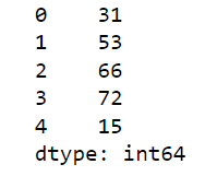
Without issue, we are able to pass our Python list as data into the Series constructor. Similar to the Python list, the pandas Series has an index that we can reference when we want to select an individual element from the series.
How to create a pandas Series from a dictionary
Besides using a list, we can pass a Python dictionary into the pandas Series constructor. Constructing a Series object using a dictionary behaves a bit differently than when a list is passed in as data..
data = {'a':1, 'b':2, 'c':3}
s = pd.Series(data)
print(s)
Looking at the, we see the dictionary’s key is set as the index. This is referred to as labeling the index.

By passing values to the index parameter inside of the Series constructor, we can manipulate the order of the index labels and add new index positions that aren’t associated with a data value.
data = {'a':1, 'b':2, 'c':3}
s = pd.Series(data, index = ['c','b','a','z'])
print(s)
Notice we added the label z to the index and the value is NaN (not a number) because it doesn’t exist in the dictionary we used to create the pandas Series.
How to select an element from a pandas Series
We can select an element of the series by referencing its index number or label. For example, if we want to return the value 2.0 from the Series, we can use either strategy since our index has a label:
#get the element by index number
print(s[1])

#get the element by  label
print(s['b'])
Either method of returning the element from the Series produces the same result.
Now that we’ve reviewed how to create a pandas Series from a list and a dictionary, we’ve established a foundation on which we can navigate indexes and select elements of data. Let’s begin to explore DataFrames and go deeper into pandas functionality.
5. Python pandas tutorial: DataFrame
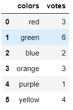
A DataFrame is a 2-dimensional object with an index that represents data stored in rows and columns. DataFrames are versatile data structures since we can perform arithmetic operations on rows and columns, pivot the data, and easily summarize it.
Let’s start the Python pandas tutorial for DataFrames by creating a pandas DataFrame from a Python dictionary using the DataFrame constructor. The syntax looks similar to the Series constructor, but takes a columns argument:
pandas.DataFrame( data, index, columns, dtype, copy)
#create a data object
data = {
  	"colors": ['red', 'green', 'blue', 'orange', 'purple', 'yellow'],
 	"votes": [3, 6, 2, 3, 1, 4],
	"cars": [1, 2, 1, 1, 2, 1]
}

#load data into a DataFrame object:
df = pd.DataFrame(data)

#display the DataFrame
df
The DataFrame output will look like this:

When the DataFrame doesn’t have many rows, they will all display in the output. When the DataFrame has many rows, only the top five and bottom 5 will display at a time by default.
How to explore a pandas DataFrame
When we load data into a pandas DataFrame, we typically want to do some exploratory analysis to better understand the data, the columns, and the descriptive statistics. Here are the six basic pandas functions used for exploring any pandas DataFrame:
Display the names of the columns in the DataFrame using .columns.
#display the columns
df.columns
Display the index range of the DataFrame using .index.
#display the index
df.index
Display the first five rows of the DataFrame using .head() and last five rows of the DataFrame using .tail(). Keep in mind that .head() and .tail() allow an integer n to be passed into it, overriding the default value of five:
#Example of n values
df.head(1) #returns top 1 row
df.tail(6) #returns last 4 rows
Display summary statistics like count, mean, min and max, for each numeric column in the DataFrame using .describe()

Notice the colors column didn’t output since it is not a numeric data type.
Display the data types of the columns in the DataFrame, the number of nulls in each column, and the DataFrame’s overall memory usage using .info().
#display data types
df.info()
How to select columns and data in a pandas DataFrame
It is possible to select one or more columns in a DataFrame and perform operations on them like aggregations, arithmetic, and transformations. For example, let’s say we only want to select the columns colors and votes from the DataFrame named df. To do this, we pass a list of column names into brackets, like we’re selecting labeled indexes from a Series.
#select specific DataFrame columns
df[['colors', 'votes']]
Beyond being able to select specific columns, there are three basic ways to select data from within the specified columns. Data can be selected in slices using brackets [ ], the .loc[ ] attribute, and the .iloc[ ] attribute.
If you’ve worked with strings and lists in Python, the syntax for slicing a dataframe should already look familiar. Keep in mind, the slice is exclusive of the last value which means it outputs a range of [x:y-1]. For example, if we want to output rows 2,3,4 we’d use a slice range of [2:5].
#slicing the DataFrame to output 2,3,4
df[['colors','votes']][2:5]
The .loc[ ] attribute is a very useful tool for indexing and slicing data in a DataFrame, and it is particularly useful when working with large datasets where it is more efficient to select rows and columns using labels rather than integer-based indexing.
The basic syntax for using the loc attribute is as follows:
DataFrame.loc[row_indexer, column_indexer]
The row_indexer is a label or list of labels used to select rows, and column_indexer is a label or list of labels used to select columns.
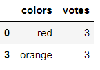
Logical operations can be done within the .loc[ ] attribute, making it an easy way to search for specific elements in the data. For example, let’s find all the colors where the vote = 3.
#find colors with 3 votes
df[['colors','votes']].loc[df['votes'] == 3]
Use DataFrame.iloc[ ] to pass index values instead of columns or rows. This is useful if you can programmatically avoid needing to use labels. For example, we can return all values for the votes column using .iloc[ ] like this:
#return the votes values using iloc[]
 df[['colors','votes']].iloc[:,1]
In general, the .loc[ ] attribute is more useful when you want to index and slice data using row and column labels, while the .iloc[ ] attribute is more useful when you want to use integer-based positions to index and slice data.
How to apply aggregate functions to a pandas DataFrame
Pandas makes it easy to generate summary statistics using operations like mean, sum, count, and more. For example, to calculate the mean of all the values in a DataFrame, you can use the mean() function. Most of the aggregate operations exclude missing data and operate across rows by default. Try counting the number of rows using the count() function:
#use .count to count the number of rows for each column
df[['colors','votes']].count()
Practice some of the other commonly used aggregate functions on the votes column.
#Use .mean() to find the mean votes
df['vote'].mean()

# Use .median() to find the median votes
df[vote].median()

# Use .mode() to find the mode votes
df['vote'].mode()

# Use .min() to find the minimum votes
df['vote'].min()

# Use .max() to find the maximum votes
df['vote'].max()
One of the main benefits of using pandas aggregate functions is that they are very easy to use and can be applied to a DataFrame with a single line of code. I recommend bookmarking the documentation’s quick reference of aggregate functions until you’ve memorized how to use them all.
How to sort, group and pivot data in a pandas DataFrame
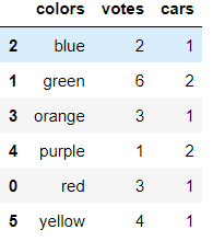
There are several ways to sort, group, and pivot data in a pandas DataFrame. While sorting is fairly straightforward (ascending and descending), grouping allows you to group the data by one or more columns and then apply an aggregation function to each group. A pivot table is similar to grouping, but requires multiple dimensions and an aggregate function.
To sort a DataFrame, you can use the sort_values() function, which allows you to sort the data by one or more columns. For example, let’s sort the DataFrame by colors alphabetically.
#sort colors in ascending order
df.sort_values('colors', ascending = True)
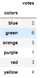
Pandas also provides the .groupby() function, which can be used when applying aggregate functions. For example, let’s group the DataFrame by the values in the colors column and calculate the .mean() of each group:
#group by colors and calc mean
df[['colors','votes']].groupby('colors').mean()
Using pandas, pivot tables can also be created in a line of code. To pivot a DataFrame, you can use the pivot_table() function, which allows you to create a pivot table that summarizes and analyzes data by grouping it into categories and calculating statistics for each group.Let’s transform the DataFrame into a pivot table using the aggregate function mean:
#create a pivot table using mean
df.pivot_table(index='colors', values=['votes', 'cars'], aggfunc='mean')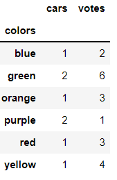
Overall, these are just a few examples of how you can sort, group, and pivot data in a pandas DataFrame. There are many other functions and techniques available in the pandas library that can help you manipulate and analyze your data.
6. Next steps
The Python pandas library is a powerful analytics tool because it can ingest many different forms of data and has easy to work with data structures like the Series and the DataFrame.
In the Python pandas tutorial, we explored several ways to slice the data structures and select specific rows or columns from them. Also, we looked at how to apply aggregate functions, sort, group and pivot the data in the data structures.
The combination of pandas efficient data structures, robust features and active developer community have made it one of the most popular open source Python analytics libraries on the market.
Now that you’ve completed this Python pandas tutorial, you’ve proven that you’re capable of doing what it takes to become a data analyst. If you’re interested in learning more about data analytics, why not try out our free, 5-day short course?
You may also be interested in the following articles:


