The SUBTOTAL function in Microsoft Excel returns the subtotal value from a range of cells. It allows you to use other functions, like AVERAGE or COUNT, to find custom totals from a dataset. We’ll explain how to use the SUBTOTAL function, step-by-step, in this tutorial.
Mathematical functions like SUM, AVERAGE, and MIN exist in their own right in Excel, allowing you to analyze data in your own way. If you want to use these functions to find subtotals, however, you can easily do this using the SUBTOTAL function.
SUBTOTAL automatically ignores any other examples of SUBTOTAL formulas, making it a better option if you’re looking to add subtotals within your dataset without impacting the data that’s reported.
You can learn more Excel analysis skills with our free 5-day data short course.
In this guide, we’ll explain:
- What is the SUBTOTAL function and what is it used for?
- How does the SUBTOTAL function work in Microsoft Excel?
- Things to consider before using SUBTOTAL in Excel
- How to use SUBTOTAL in an Excel formula: A step-by-step guide
Are you thinking about using the SUBTOTAL function to analyze your spreadsheet data? To help, we’ll explain how it works and how to use it effectively.
1. What is the SUBTOTAL function and what is it used for?
At first glance, you might wonder: what is the point of the SUBTOTAL function? After all, it’s easy enough to find a subtotal from a range of cells using existing functions like SUMIF or AVERAGE.
While it’s true that you don’t necessarily need to use SUBTOTAL, it makes targeted data analysis a lot easier. You can insert a formula using SUBTOTAL into a range of cells without it affecting the overall total, because SUBTOTAL ignores other cells that contain a SUBTOTAL formula.
SUBTOTAL works with other Excel features, such as cell filtering. If you filter a table using a value, the SUBTOTAL formula updates, recognizing the filter and excluding cells accordingly. SUBTOTAL is also useful for ignoring hidden values, which other functions (like SUM) can’t do.
Thankfully, you can use other functions as part of a SUBTOTAL formula. 11 different subtotal methods are available, each matching an existing Excel function. If you want a SUM formula that works with filtered cells and ignores other SUBTOTAL formulas, then using SUBTOTAL is best, although a pivot table could work in a similar way.
2. How does the SUBTOTAL function work in Microsoft Excel?
The SUBTOTAL function works by calculating the total value of a cell range, based on another mathematical function.
SUBTOTAL uses up to 11 different mathematical functions (from AVERAGE to VAR.P) to find the right total value, while working within the parameters of the function (ignoring other SUBTOTAL formulas, for instance).
A SUBTOTAL formula is easily created using the following structure:
=SUBTOTAL(function_num, ref1, ref2,…)
A formula using SUBTOTAL has at least two arguments: function_num and ref1. Further arguments,starting with ref2, are optional. In this example formula, the function_num argument refers to the function you wish to use with SUBTOTAL.
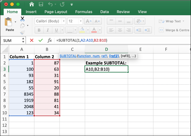
As we’ve mentioned, 11 different functions are available, but you can’t use =SUBTOTAL(SUM, and expect it to work. Instead, you’ll need to use a number to represent the function you wish to use. These are:
- 1 or 101: AVERAGE
- 2 or 102: COUNT
- 3 or 103: COUNTA
- 4 or 104: MAX
- 5 or 105: MIN
- 6 or 106: PRODUCT
- 7 or 107: STDEV
- 8 or 108: STDEVP
- 9 or 109: SUM
- 10 or 110: VAR
- 11 or 111: VARP
The variations in number determine whether SUBTOTAL includes or ignores hidden numbers. Using the numbers 1-11 allows SUBTOTAL to include numbers from hidden rows or columns, while using 101-111 allows SUBTOTAL to exclude them.
The ref1 argument is required, as this is the initial range of cells that you’ll want to subtotal using one of the 11 functions. If you want to take this further, you can add up to 254 different cell ranges, one by one. This will create a combined subtotal using the total data across all the included cell ranges.
3. Things to consider before using SUBTOTAL in Excel
While SUBTOTAL has advantages, there are also a few things you’ll need to consider before you start using it. These include:
- As mentioned, using 1-11 for the function_num argument will ensure that SUBTOTAL includes hidden values, while 101-111 ignores them.
- Using a value other than 1-11 or 101-111 will cause Excel to return a #VALUE! Error. This will also occur for 3D cell references (where the same cell, across multiple worksheets, is referenced in a range).
- When horizontal cell ranges like A1:D1 are used, hidden values are included automatically (regardless of the function_num argument value). This is a limitation of the SUBTOTAL function and can’t be overcome.
- Using SUBTOTAL on filtered data will ensure that hidden values are always ignored, regardless of the function_num argument used.
- SUBTOTAL can be used as a nested function as part of other functions, including formulas containing the IF function.
- If another SUBTOTAL formula is within the ref1 data range, then SUBTOTAL will ignore it and exclude it from the overall calculation.
- Excel allows a maximum of 254 cell ranges to be used in a SUBTOTAL formula, although only 1 is required for the formula to work.
4. How to use SUBTOTAL in an Excel formula: A step-by-step guide
If you want to create a SUBTOTAL formula in Microsoft Excel, you’ll need to follow these steps:
Step 1: Select an empty cell
Start by opening your Excel spreadsheet (containing your data) and selecting an empty cell. Once selected, press the formula bar and ensure that the blinking cursor is active.
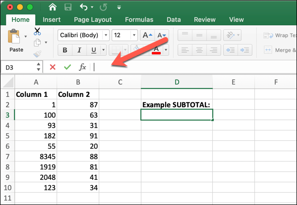
From here, you can begin to craft your new SUBTOTAL formula.
Step 2: Insert the function_num method
Next, you’ll need to begin creating your new SUBTOTAL formula using the syntax and structure outlined above. Begin by typing =SUBTOTAL( in the formula bar.
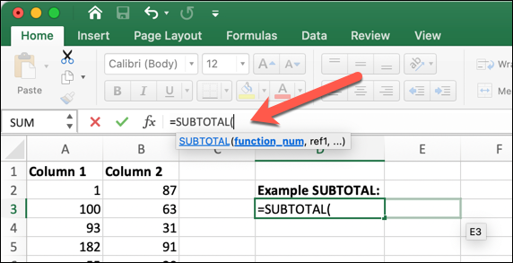
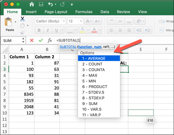
The first component of a SUBTOTAL formula is the function_num method, which correlates to another Excel mathematical function. To do this, type a number from 1 to 11 to create a SUBTOTAL formula that includes hidden values, or 101 to 111 to create a formula that ignores them.
For instance, =SUBTOTAL(101 will use the AVERAGE function to show the average from the cell range selected, excluding any hidden values. When you begin to type a SUBTOTAL formula, an options menu will appear below the formula, allowing you to select one of these methods automatically.
When we refer to hidden values, we mean cells that exist in columns that are hidden.
This excludes filtered data (which is always hidden) or SUBTOTALs using horizontal cell ranges (where the values are always shown).
Step 3: Select your SUBTOTAL ranges
At the next stage, you’ll need to specify the required ref2 cell range.
This is the data that the SUBTOTAL formula will use to calculate a subtotal. If you want to create a subtotal using multiple cell ranges, you can add these (one after another) after the function_num method is specified.
For example, if you wanted to count the number of cells in ranges A2:A9 and B2:B9, use the formula =SUBTOTAL(102,A2:A9,B2:B9), making sure to close the formula with a closing parentheses.
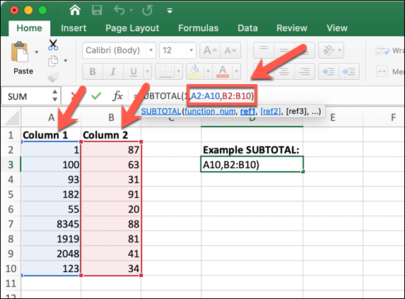
If the range contains invalid data (for example, a text string), then Excel will return an error message. You’ll need to remove the conflicting data or change the data range used in your SUBTOTAL formula to resolve this.
Final thoughts
Using the SUBTOTAL function can help you quickly analyze datasets without relying on more complex pivot tables.
If you’re struggling, you can also use the Subtotal feature, found in the Data tab in the ribbon bar, to automatically generate a SUBTOTAL formula which you can then edit or copy elsewhere.
Excel formulas are just one of many key skills needed in the data analytics field. For a hands-on introduction to data analysis, give CareerFoundry’s free introductory short course a try. You can learn more about the skills and techniques you’ll need to become a data analyst in the following posts:
