The SUMPRODUCT function in Excel is a very powerful function.
It is a very versatile Excel function and has special powers that are of particular interest to users of Excel versions prior to Excel 365.
The SUMPRODUCT function returns the sum of the products of the corresponding ranges or arrays. Its most common use is to sum or count values based on multiple criteria. This makes it a very useful function for data analysis in Excel.
In this tutorial, we’ll show you how to use the SUMPRODUCT function. This will be supported by a few examples to showcase its versatility.
You can learn more Excel analysis skills with CareerFoundry’s free 5-day data short course.
This tutorial will cover:
- What is the SUMPRODUCT function and why use it?
- How to use the SUMPRODUCT function (step-by-step)
- Things to remember when using the SUMPRODUCT function
- Sum values that meet specific criteria
- Sum values that meet multiple criteria
- SUMPRODUCT working with arrays
- Key takeaways
Download the Excel workbook and follow along with the examples in this tutorial.
So: let’s dive into the SUMPRODUCT function.
1. What is the SUMPRODUCT function and why use it?
The SUMPRODUCT function is available for all versions of Excel and has secret powers that bring joy to users when they first learn it.
It sums the products of given ranges or arrays. However, other operations such as addition can also be applied.
It is most well-known for its ability to handle multiple criteria when performing aggregations such as sum or count. If you’re using Excel for data analysis, then this function is incredibly useful.
The SUMPRODUCT function requires only the arrays that you want to multiply and then sum. It can handle up to 255 arrays. These ranges or arrays must be the same size.
=SUMPRODUCT(array1, [array2], [array3], …)
2. How to use the SUMPRODUCT function in Excel (step-by-step)
Let’s start with a simple example of SUMPRODUCT performing the role of summing the product of two arrays.
In the image below, we have 5 events along with the quantity sold and the ticket price.
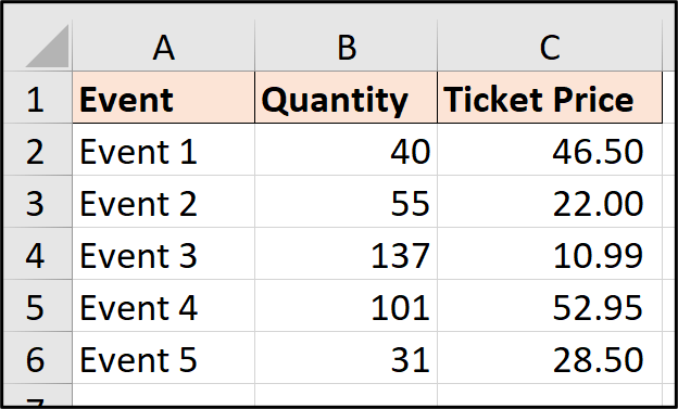
We would like to return the total revenue of ticket sales. In the following image, the total for each row is calculated using the formula B2*C2 and so on for each row from cell D2.
A SUM function is then used in cell D8 to total the values in range D2:D6. This is a common Excel approach to finding the total revenue.
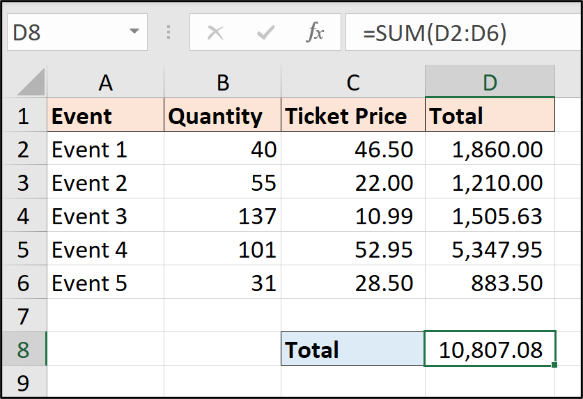
This approach is great, and possibly better if you wanted the total for each row. However, SUMPRODUCT can achieve this in one formula, eliminating the requirement to create those row totals first.
The following formula is used in cell C8 to return the total ticket sales revenue with just one formula.
=SUMPRODUCT(B2:B6,C2:C6)
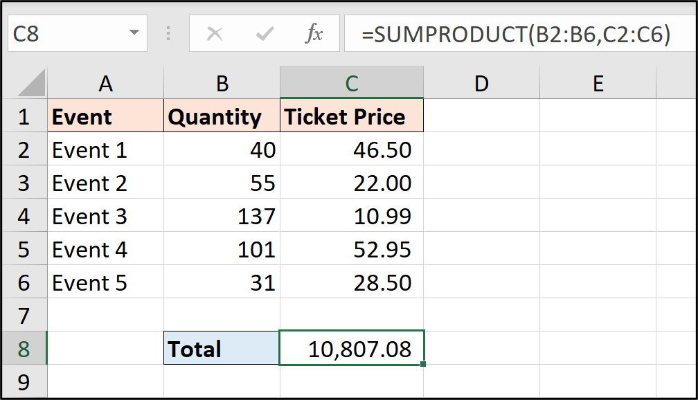
The SUMPRODUCT function is provided with the two arrays. That is all that it needs.
It multiplies the values from the corresponding ranges together i.e. B2*C2, B3*C3 and so on, stores the results in an array i.e. {1860, 1210 …}, then the values are summed to return the final result of 10,807.08.
3. Things to remember when using the SUMPRODUCT function
There are a few important things to remember when using SUMPRODUCT:
- The dimensions of each range or array must be the same.
- It is recommended to avoid the use of whole column references such as B:B. In this tutorial, table references are used. These are a superior method of referencing.
- The double unary (–) can be used to convert TRUE and FALSE values to 1 and 0 respectively.
- When working with multiple criteria, the asterix (*) is used for AND logic and the plus operator (+) is used for OR logic.
4. Sum values that meet specific criteria
The SUMPRODUCT function is used for many reasons as it is such a versatile function. Summing and counting values that meet specific criteria is its most popular use.
Let’s begin with an example that includes a single criteria, and then move on to see SUMPRODUCT work with multiple criteria.
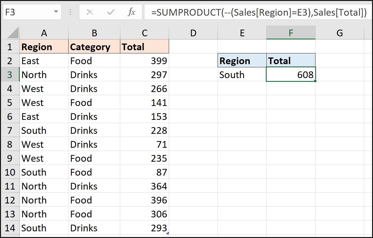
The following image shows a table named ‘Sales’ with columns for the Region, Category, and a Total. We will use SUMPRODUCT to return the total of all values for the region in cell E3.
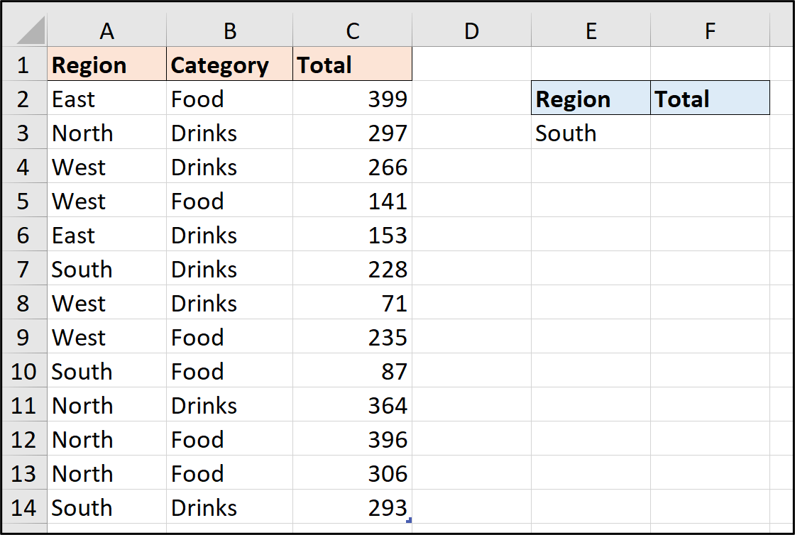
The following formula is used in cell F3.
=SUMPRODUCT(–(Sales[Region]=E3),Sales[Total])
It tests if the values in the ‘Region’ column are equal to the value in cell E3. These results are returned as TRUE and FALSE values, so the test is enclosed in brackets and the double unary (–) is used to convert these to 1 and 0.
The 1s and 0s are multiplied by the corresponding value in the ‘Total’ range and then summed to return the final result.
As an alternative to the double unary, the bracketed criteria could be multiplied by the ‘Total’ range. The multiply operation will convert the test result to 1s and 0s.
=SUMPRODUCT((Sales[Region]=E3)*Sales[Total])
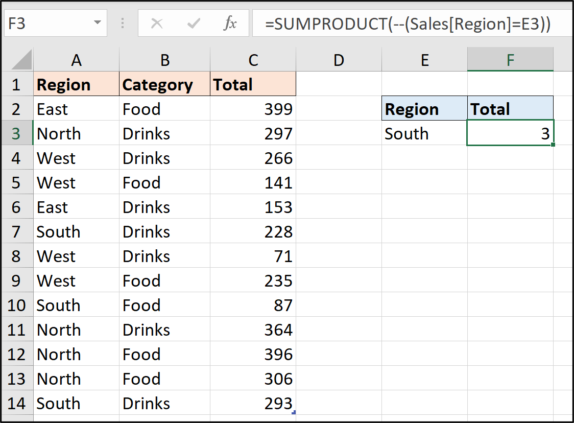
Finally, to change the sum to a count, you just need to remove the ‘Total’ column from the second array. This is shown in the following formula.
=SUMPRODUCT(–(Sales[Region]=E3))
5. Sum values that meet multiple criteria
As mentioned already, the SUMPRODUCT function is most well-known for its ability to handle multiple criteria.
It can sum and count values with ease, and also work with both AND and OR logic. This is especially impressive as the COUNTIFS and SUMIFS functions only work with AND logic.
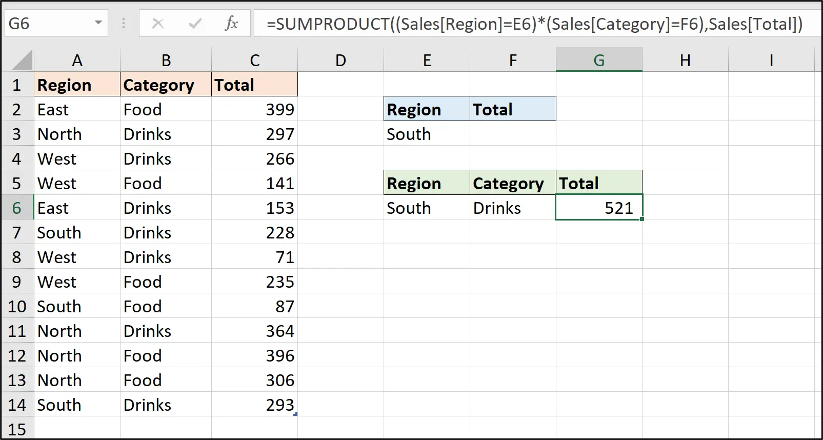
Continuing with the same dataset, the following formula is used to sum the total values when the region is equal to that entered in cell E6, and the category is equal to that entered in cell F6.
=SUMPRODUCT((Sales[Region]=E6)*(Sales[Category]=F6),Sales[Total])
Each criteria is enclosed in its own set of brackets and the asterisk (*) is used to multiply the two arrays. The asterisk can be thought of as the AND operator in SUMPRODUCT.
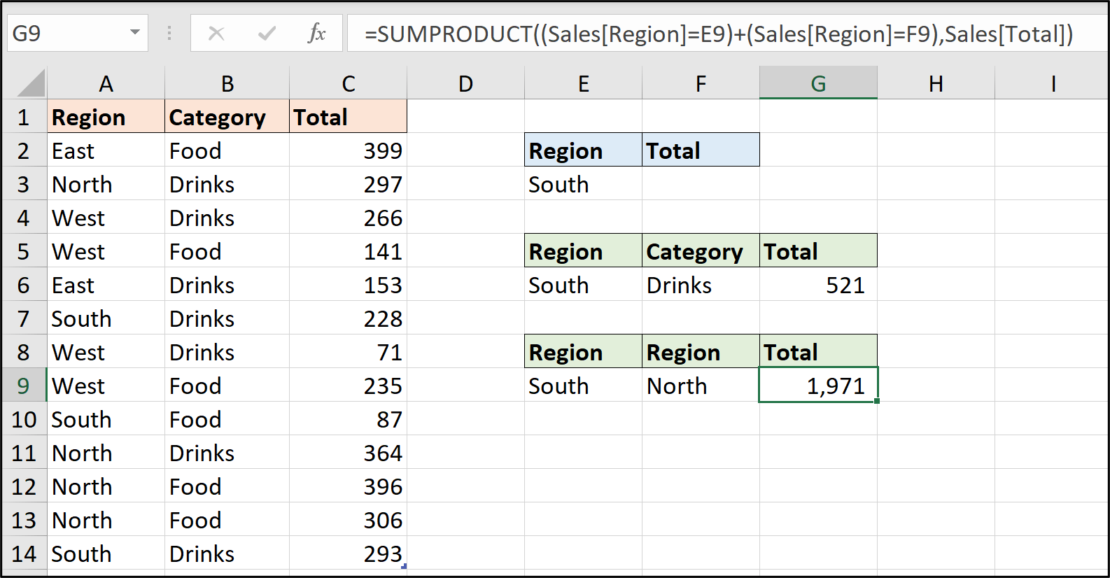
To apply OR logic, the plus operator (+) is used.
The following formula sums the total values when the region is equal to the one entered into cell E9 or F9.
=SUMPRODUCT((Sales[Region]=E9)+(Sales[Region]=F9),Sales[Total])
6. SUMPRODUCT working with arrays
SUMPRODUCT makes it easy to work with arrays. This makes it a very important function for Excel versions prior to Excel 365 as they do not have the array engine found in modern Excel.
Using SUMPRODUCT avoids the requirement to press Ctrl + Shift + Enter when running array formulas.
In this final example, we have a table named ‘Locations’ with Reference and Total columns.
The following formula is entered into cell E3 to sum the values for the reference that ends in the three characters entered into cell D3.
=SUMPRODUCT(–(RIGHT(Locations[Reference],3)=D3),Locations[Total])
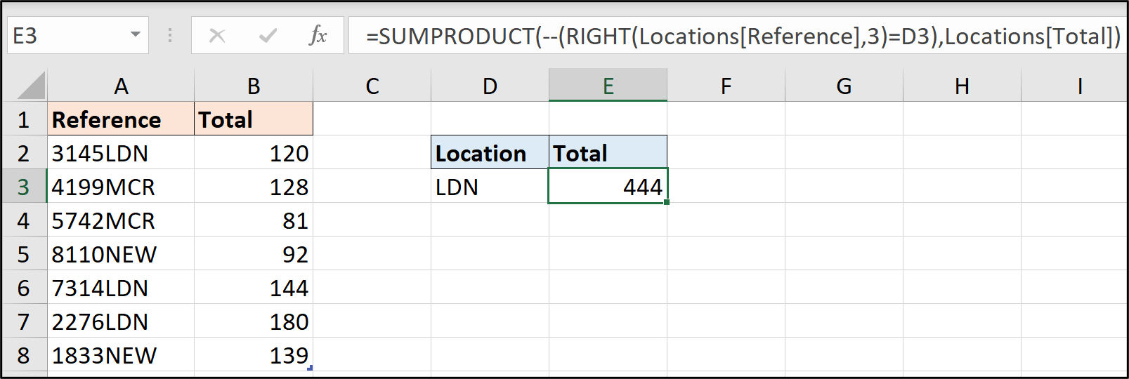
The formula uses the RIGHT function to extract the last three characters from the values in the ‘Reference’ column. These are then tested against the value in cell D3.
The SUMIFS function would not allow the use of RIGHT nested within itself. So, this example gives further insight to the power of SUMPRODUCT and why it is so highly valued by advanced Excel users.
7. Final thoughts
Excel formulas are an extremely handy tool for anyone working with data—especially data analysts. For a hands-on introduction to the field of data analytics, try out this free five-day short course. And, for more Excel tutorials, check out the following:
