What is ordinal data, how is it used, and how do you collect and analyze it? Find out in this comprehensive guide.
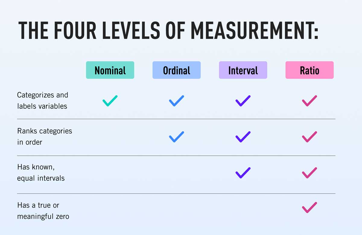
Whether you’re new to data analytics or simply need a refresher on the fundamentals, a key place to start is with the four types of data. Also known as the four levels of measurement, this data analytics term describes the level of detail and precision with which data is measured. The four types (or scales) of data are:
- nominal data
- ordinal data
- interval data
- ratio data
In this article, I’m going to dive deep into ordinal data.
If the concept of these data types is completely new to you, we’ll start with a quick summary of the four different types, and then explore the various aspects of ordinal data in a bit more detail,
If you’d like to learn more data analytics skills, try our free 5-day data short course.
I’ll cover the following topics:
- An introduction to the four different types of data
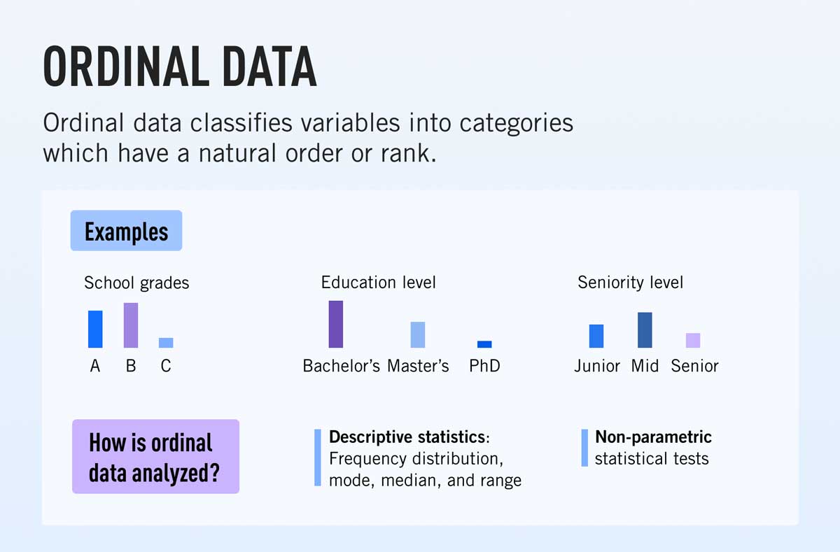
- What is ordinal data? A definition
- What are some examples of ordinal data?
- How is ordinal data collected and what is it used for?
- How to analyze ordinal data
- Summary and further reading
Ready to get your head around ordinal data? Then let’s get going!
1. An introduction to the four different types of data
To analyze a dataset, you first need to determine what type of data you’re dealing with.
Fortunately, to make this easier, all types of data fit into one of four broad categories: nominal, ordinal, interval, and ratio data. While these are commonly referred to as ‘data types,’ they are really different scales or levels of measurement.
Each level of measurement indicates how precisely a variable has been counted, determining the methods you can use to extract information from it. The four data types are not always clearly distinguishable; rather, they belong to a hierarchy. Each step in the hierarchy builds on the one before it.

The first two types of data, known as categorical data, are nominal and ordinal. These two scales take relatively imprecise measures.
While this makes them easier to analyze, it also means they offer less accurate insights. The next two types of data are interval and ratio. These are both types of numerical data, which makes them more complex. They are more difficult to analyze but have the potential to offer much richer insights.
- Nominal data is the simplest data type. It classifies data purely by labeling or naming values e.g. measuring marital status, hair, or eye color. It has no hierarchy to it.
- Ordinal data classifies data while introducing an order, or ranking. For instance, measuring economic status using the hierarchy: ‘wealthy’, ‘middle income’ or ‘poor.’ However, there is no clearly defined interval between these categories.
- Interval data classifies and ranks data but also introduces measured intervals. A great example is temperature scales, in Celsius or Fahrenheit. However, interval data has no true zero, i.e. a measurement of ‘zero’ can still represent a quantifiable measure (such as zero Celsius, which is simply another measure on a scale that includes negative values).
- Ratio data is the most complex level of measurement. Like interval data, it classifies and ranks data, and uses measured intervals. However, unlike interval data, ratio data also has a true zero. When a variable equals zero, there is none of this variable. A good example of ratio data is the measure of height—you cannot have a negative measure of height.
You’ll find a comprehensive guide to the four levels of data measurement here.
What do the different levels of measurement tell you?
Distinguishing between the different levels of measurement is sometimes a little tricky.
However, it’s important to learn how to distinguish them, because the type of data you’re working with determines the statistical techniques you can use to analyze it. Data analysis involves using descriptive analytics (to summarize the characteristics of a dataset) and inferential statistics (to infer meaning from those data).
These comprise a wide range of analytical techniques, so before collecting any data, you should decide which level of measurement is best for your intended purposes.
2. What is ordinal data? A definition
Ordinal data is a type of qualitative (non-numeric) data that groups variables into descriptive categories.
A distinguishing feature of ordinal data is that the categories it uses are ordered on some kind of hierarchical scale, e.g. high to low. On the levels of measurement, ordinal data comes second in complexity, directly after nominal data.

While ordinal data is more complex than nominal data (which has no inherent order) it is still relatively simplistic.
For instance, the terms ‘wealthy’, ‘middle income’, and ‘poor’ may give you a rough idea of someone’s economic status, but they are an imprecise measure–there is no clear interval between them. Nevertheless, ordinal data is excellent for ‘sticking a finger in the wind’ if you’re taking broad measures from a sample group and fine precision is not a requirement.
While ordinal data is non-numeric, it’s important to understand that it can still contain numerical figures. However, these figures can only be used as categorizing labels, i.e. they should have no inherent mathematical value.
For instance, if you were to measure people’s economic status you could use number 3 as shorthand for ‘wealthy’, number 2 for ‘middle income’, and number 1 for ‘poor.’ At a glance, this might imply numerical value, e.g. 3 = high and 1 = low. However, the numbers are only used to denote sequence. You could just as easily switch 3 with 1, or with ‘A’ and ‘B’ and it would not change the value of what you’re ordering; only the labels used to order it.
Key characteristics of ordinal data
- Ordinal data are categorical (non-numeric) but may use numbers as labels.
- Ordinal data are always placed into some kind of hierarchy or order (hence the name ‘ordinal’—a good tip for remembering what makes it unique!)
- While ordinal data are always ranked, the values do not have an even distribution.
- Using ordinal data, you can calculate the following summary statistics: frequency distribution, mode and median, and the range of variables.
What’s the difference between ordinal data and nominal data?
While nominal and ordinal data are both types of non-numeric measurement, nominal data have no order or sequence.
For instance, nominal data may measure the variable ‘marital status,’ with possible outcomes ‘single’, ‘married’, ‘cohabiting’, ‘divorced’ (and so on). However, none of these categories are ‘less’ or ‘more’ than any other. Another example might be eye color. Meanwhile, ordinal data always has an inherent order.
If a qualitative dataset lacks order, you know you’re dealing with nominal data.
3. What are some examples of ordinal data?
What are some examples of ordinal data?
- Economic status (poor, middle income, wealthy)
- Income level in non-equally distributed ranges ($10K-$20K, $20K-$35K, $35K-$100K)
- Course grades (A+, A-, B+, B-, C)
- Education level (Elementary, High School, College, Graduate, Post-graduate)
- Likert scales (Very satisfied, satisfied, neutral, dissatisfied, very dissatisfied)
- Military ranks (Colonel, Brigadier General, Major General, Lieutenant General)
- Age (child, teenager, young adult, middle-aged, retiree)
As is hopefully clear by now, ordinal data is an imprecise but nevertheless useful way of measuring and ordering data based on its characteristics. Next up, let’s see how ordinal data is collected and how it generally tends to be used.
4. How is ordinal data collected and what is it used for?
Ordinal data are usually collected via surveys or questionnaires. Any type of question that ranks answers using an explicit or implicit scale can be used to collect ordinal data. An example might be:
- Question: Which best describes your knowledge of the Python programming language? Possible answers: Beginner, Basic, Intermediate, Advanced, Expert.
This commonly recognized type of ordinal question uses the Likert Scale, which we described briefly in the previous section. Another example might be:
- Question: To what extent do you agree that data analytics is the most important job for the 21st century? Possible answers: Strongly agree, Agree, Neutral, Disagree, Strongly Disagree.
It’s worth noting that the Likert Scale is sometimes used as a form of interval data. However, this is strictly incorrect. That’s because Likert Scales use discrete values, while interval data uses continuous values with a precise interval between them.
The distinctions between values on an ordinal scale, meanwhile, lack clear definition or separation, i.e. they are discrete. Although this means the values are imprecise and do not offer granular detail about a population, they are an excellent way to draw easy comparisons between different values in a sample group.
How is ordinal data used?
Ordinal data are commonly used for collecting demographic information.
This is particularly prevalent in sectors like finance, marketing, and insurance, but it is also used by governments, e.g. the census, and is generally common when conducting customer satisfaction surveys (in any industry).
5. How to analyze ordinal data
As discussed, the level of measurement you use determines the kinds of analysis you can carry out on your data. In general, these fall into two broad categories: descriptive statistics and inferential statistics.
We use descriptive statistics to summarize the characteristics of a dataset. This helps us spot patterns. Meanwhile, inferential statistics allow us to make predictions (or infer future trends) based on existing data. However, depending on the measurement scale, there are limits. You can learn more about the difference between descriptive and inferential statistics here.
For now, though, Let’s see what kinds of descriptive and inferential statistics you can measure using ordinal data.
Descriptive statistics for ordinal data
The descriptive statistics you can obtain using ordinal data are:
- Frequency distribution
- Measures of central tendency: Mode and/or median
- Measures of variability: Range
Now let’s look at each of these in more depth.
Frequency distribution
Frequency distribution describes how your ordinal data are distributed.
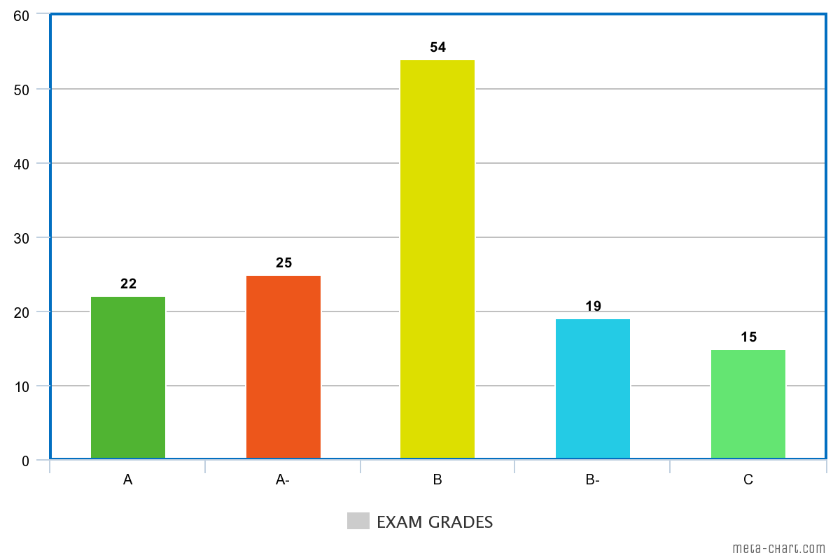
For instance, let’s say you’ve surveyed students on what grade they’ve received in an examination. Possible grades range from A to C. You can summarize this information using a pivot table or frequency table, with values represented either as a percentage or as a count. To illustrate using a very simple example, one such table might look like this:

As you can see, the values in the sum column show how many students received each possible grade. This allows you to see how the values are distributed. Another option is also to visualize the data, for instance using a bar plot.

Viewing the data visually allows us to easily see the frequency distribution. Note the hierarchical relationship between categories. This is different from the other type of categorical data, nominal data, which lacks any hierarchy.
Measures of central tendency: Mode and/or median
The mode (the value which is most often repeated) and median (the central value) are two measures of what is known as ‘central tendency.’ There is also a third measure of central tendency: the mean. However, because ordinal data is non-numeric, it cannot be used to obtain the mean. That’s because identifying the mean requires mathematical operations that cannot be meaningfully carried out using ordinal data.
However, it is always possible to identify the mode in an ordinal dataset. Using the barplot or frequency table, we can easily see that the mode of the different grades is B. This is because B is the grade that most students received.
In this case, we can also identify the median value. The median value is the one that separates the top half of the dataset from the bottom half. If you imagined all the respondents’ answers lined up end-to-end, you could then identify the central value in the dataset. With 165 responses (as in our grades example) the central value is the 83rd one. This falls under the grade B.
Measures of variability: Range
The range is one measure of what is known as ‘variability.’ Other measures of variability include variance and standard deviation. However, it is not possible to measure these using ordinal data, for the same reasons you cannot measure the mean.
The range describes the difference between the smallest and largest value. To calculate this, you first need to use numeric codes to represent each grade, i.e. A = 1, A- = 2, B = 3, etc. The range would be 5 – 1 = 4. So in this simple example, the range is 4. This is an easy calculation to carry out. The range is useful because it offers a basic understanding of how spread out the values in a dataset are.
Inferential statistics for ordinal data
Descriptive statistics help us summarize data. To infer broader insights, we need inferential statistics. Inferential statistics work by testing hypotheses and drawing conclusions based on what we learn.
There are two broad types of techniques that we can use to do this. Parametric and non-parametric tests. For qualitative (rather than quantitative) data like ordinal and nominal data, we can only use non-parametric techniques.
Non-parametric approaches you might use on ordinal data include:
- Mood’s median test
- The Mann-Whitney U test
- Wilcoxon signed-rank test
- The Kruskal-Wallis H test:
- Spearman’s rank correlation coefficient
Let’s briefly look at these now.
Mood’s median test
The Mood’s median test lets you compare medians from two or more sample populations in order to determine the difference between them. For example, you may wish to compare the median number of positive reviews of a company on Trustpilot versus the median number of negative reviews. This will help you determine if you’re getting more negative or positive reviews.
The Mann-Whitney U-test
The Mann-Whitney U test lets you compare whether two samples come from the same population.
It can also be used to identify whether or not observations in one sample group tend to be larger than observations in another sample. For example, you could use the test to understand if salaries vary based on age. Your dependent variable would be ‘salary’ while your independent variable would be ‘age’, with two broad groups, e.g. ‘under 30,’ ‘over 60.’
Wilcoxon signed-rank test
The Wilcoxon signed-rank test explores the distribution of scores in two dependent data samples (or repeated measures of a single sample) to compare how, and to what extent, the mean rank of their populations differs.
We can use this test to determine whether two samples have been selected from populations with an equal distribution or if there is a statistically significant difference.
The Kruskal-Wallis H test
The Kruskal-Wallis H test helps us to compare the mean ranking of scores across three or more independent data samples.
It’s an extension of the Mann-Whitney U test that increases the number of samples to more than two. In the Kruskal-Wallis H test, samples can be of equal or different sizes. We can use it to determine if the samples originate from the same distribution.
Spearman’s rank correlation coefficient
Spearman’s rank correlation coefficient explores possible relationships (or correlations) between two ordinal variables.
Specifically, it measures the statistical dependence between those variable’s rankings. For instance, you might use it to compare how many hours someone spends a week on social media versus their IQ. This would help you to identify if there is a correlation between the two.
Don’t worry if these models are complex to get your head around. At this stage, you just need to know that there are a wide range of statistical methods at your disposal. While this means there is lots to learn, it also offers the potential for obtaining rich insights from your data.
6. Summary and further reading
In this guide, we:
- Introduced the four levels of data measurement: Nominal, ordinal, interval, and ratio.
- Defined ordinal data as a qualitative (non-numeric) data type that groups variables into ranked descriptive categories.
- Explained the difference between ordinal and nominal data: Both are types of categorical data. However, nominal data lacks hierarchy, whereas ordinal data ranks categories using discrete values with a clear order.
- Shared some examples of nominal data: Likert scales, education level, and military rankings.
- Highlighted the descriptive statistics you can obtain using ordinal data: Frequency distribution, measures of central tendency (the mode and median), and variability (the range).
- Introduced some non-parametric statistical tests for analyzing ordinal data, e.g. Mood’s median test and the Kruskal-Wallis H test.
Want to learn more about data analytics or statistics? To further develop your understanding, check out our free-five day data analytics short course and read the following guides:
